Skip Connections in Transformer Models

Transformer models consist of stacked transformer layers, each containing an attention sublayer and a feed-forward sublayer. These sublayers are not directly connected; instead, skip connections combine the input with the processed output in each sublayer. In this post, you will explore skip connections in transformer models. Specifically:

• Why skip connections are essential for training deep transformer models
• How residual connections enable gradient flow and prevent vanishing gradients
• The differences between pre-norm and post-norm transformer architectures

Let’s get started.

Overview

This post is divided into three parts; they are:

• Why Skip Connections are Needed in Transformers
• Implementation of Skip Connections in Transformer Models
• Pre-norm vs Post-norm Transformer Architectures

Why Skip Connections are Needed in Transformers

Transformer models, like other deep learning models, stack many layers on top of each other. As the number of layers increases, training becomes increasingly difficult due to the vanishing gradient problem. When gradients flow backward through many layers, they can become exponentially small, making it nearly impossible for early layers to learn effectively.

The key to successful deep learning models is maintaining good gradient flow. Skip connections, also known as residual connections, create direct paths for information and gradients to flow through the network. They allow the model to learn residual functions, the difference between the desired output and the input, rather than learning complete transformations from scratch. This concept was first introduced in the ResNet paper. Mathematically, this means:

$$y = F(x) + x$$

where the function $F(x)$ is learned. Notice that setting $F(x) = 0$ makes the output $y$ equal to the input $x$. This is called identity mapping. Starting from this baseline, the model can gradually shape $y$ away from $x$ rather than searching for a completely new function $F(x)$. This is the motivation for using skip connections.

During backpropagation, the gradient with respect to the input becomes:

$$\frac{\partial L}{\partial x} = \frac{\partial L}{\partial y} \cdot \frac{\partial y}{\partial x} = \frac{\partial L}{\partial y} \cdot \left(\frac{\partial F(x)}{\partial x} + 1\right)$$

The “+1” term ensures the gradient doesn’t diminish even when $\partial F/\partial x$ is small. This is why skip connections mitigate the vanishing gradient problem.

In transformer models, skip connections are applied around each sublayer (attention and feed-forward networks). This design provides a path for gradients to flow backward, enabling transformer models to converge faster: a crucial advantage given their typically deep architecture and long training times.

The figure below illustrates typical skip connection usage:

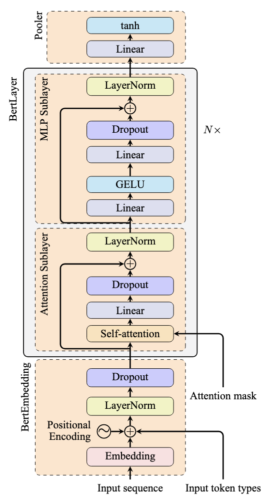
Note how the arrows represent skip connections that bypass the attention and feed-forward sublayers. These connections add the input directly to the output of each sublayer, creating a residual learning framework.

Implementation of Skip Connections in Transformer Models

Here’s how residual connections are typically implemented in transformer models:

This PyTorch implementation represents one layer of the BERT model, as illustrated in the previous figure. The nn.MultiheadAttention module replaces the self-attention and linear layers in the attention sublayer.

In the forward() method, the attention module output is saved as attn_output and added to the input x before applying layer normalization. This addition implements the skip connection. Similarly, in the MLP sublayer, the input x (the input to the MLP sublayer, not the entire transformer layer) is added to mlp_output.

Pre-norm vs Post-norm Transformer Architectures

The placement of layer normalization relative to skip connections significantly impacts training stability and model performance. Two main architectures have emerged: pre-norm and post-norm transformers.

The original “Attention Is All You Need” paper used post-norm architecture, where layer normalization is applied after the residual connection. The code above implements the post-norm architecture, applying normalization after the skip connection addition.

Most modern transformer models use pre-norm architecture instead, where normalization is applied before the sublayer:

In this pre-norm implementation, normalization is applied to the input x before the attention and MLP operations, with skip connections applied afterward.

The choice between pre-norm and post-norm architectures affects training and performance:

• Training Stability: Post-norm can be unstable during training, especially for very deep models, as gradient variance can grow exponentially with depth. Pre-norm models are more robust to train.
• Convergence Speed: Pre-norm models generally converge faster and are less sensitive to learning rate choices. Post-norm models require carefully designed learning rate scheduling and warm-up periods.
• Model Performance: Despite training challenges, post-norm models typically perform better when successfully trained.

Most modern transformer models use pre-norm architecture because they are too deep and large. In these cases, faster convergence is more valuable than slightly better performance.

Further Readings

Below are some resources that you may find useful:

Summary

In this post, you learned about skip connections in transformer models. Specifically, you learned about:

• Why skip connections are essential for training deep transformer models
• How residual connections enable gradient flow and prevent vanishing gradients
• The differences between pre-norm and post-norm transformer architectures
• When to use each architectural variant based on your specific requirements

Skip connections are a fundamental component that enables the training of very deep transformer models. The choice between pre-norm and post-norm architectures can significantly impact training stability and model performance, with pre-norm being the preferred choice for most modern applications.