Large Language Models (LLMs) can produce varied, creative, and sometimes surprising outputs even when given the same prompt. This randomness is not a bug but a core feature of how the model samples its next token from a probability distribution. In this article, we break down the key sampling strategies and demonstrate how parameters such as temperature, top-k, and top-p influence the balance between consistency and creativity.
In this tutorial, we take a hands-on approach to understand:
- How logits become probabilities
- How temperature, top-k, and top-p sampling work
- How different sampling strategies shape the model’s next-token distribution
By the end, you will understand the mechanics behind LLM inference and be able to adjust the creativity or determinism of the output.
Let’s get started.
How LLMs Choose Their Words: A Practical Walk-Through of Logits, Softmax and Sampling
Photo by Colton Duke. Some rights reserved.
Overview
This article is divided into four parts; they are:
- How Logits Become Probabilities
- Temperature
- Top-k Sampling
- Top-p Sampling
How Logits Become Probabilities
When you ask an LLM a question, it outputs a vector of logits. Logits are raw scores the model assigns to each possible next token in its vocabulary.
If the model has a vocabulary of $V$ tokens, it will output a vector of $V$ logits for each next word position. A logit is a real number. It is converted into a probability by the softmax function:
$$
p_i = \frac{e^{x_i}}{\sum_{j=1}^{V} e^{x_j}}
$$
where $x_i$ is the logit for token $i$ and $p_i$ is the corresponding probability. Softmax transforms these raw scores into a probability distribution. All $p_i$ are positive, and their sum is 1.
Suppose we give the model this prompt:
Today’s weather is so ___
The model considers every token in its vocabulary as a possible next word. For simplicity, let’s say there are only 6 tokens in the vocabulary:
|
wonderful cloudy nice hot gloomy delicious |
The model produces one logit for each token. Here’s an example set of logits the model might output and the corresponding probabilities based on the softmax function:
| Token | Logit | Probability |
|---|---|---|
| wonderful | 1.2 | 0.0457 |
| cloudy | 2.0 | 0.1017 |
| nice | 3.5 | 0.4556 |
| hot | 3.0 | 0.2764 |
| gloomy | 1.8 | 0.0832 |
| delicious | 1.0 | 0.0374 |
You can confirm this by using the softmax function from PyTorch:
|
import torch import torch.nn.functional as F
vocab = [“wonderful”, “cloudy”, “nice”, “hot”, “gloomy”, “delicious”] logits = torch.tensor([1.2, 2.0, 3.5, 3.0, 1.8, 1.0]) probs = F.softmax(logits, dim=–1) print(probs) # Output: # tensor([0.0457, 0.1017, 0.4556, 0.2764, 0.0832, 0.0374]) |
Based on this result, the token with the highest probability is “nice”. LLMs don’t always select the token with the highest probability; instead, they sample from the probability distribution to produce a different output each time. In this case, there’s a 46% probability of seeing “nice”.
If you want the model to give a more creative answer, how can you change the probability distribution such that “cloudy”, “hot”, and other answers would also appear more often?
Temperature
Temperature ($T$) is a model inference parameter. It is not a model parameter; it is a parameter of the algorithm that generates the output. It scales logits before applying softmax:
$$
p_i = \frac{e^{x_i / T}}{\sum_{j=1}^{V} e^{x_j / T}}
$$
You can expect the probability distribution to be more deterministic if $T<1$, since the difference between each value of $x_i$ will be exaggerated. On the other hand, it will be more random if $T>1$, as the difference between each value of $x_i$ will be reduced.
Now, let’s visualize this effect of temperature on the probability distribution:
|
1 2 3 4 5 6 7 8 9 10 11 12 13 14 15 16 17 18 19 20 21 22 23 24 25 |
import matplotlib.pyplot as plt import torch import torch.nn.functional as F
vocab = [“wonderful”, “cloudy”, “nice”, “hot”, “gloomy”, “delicious”] logits = torch.tensor([1.2, 2.0, 3.5, 3.0, 1.8, 1.0]) # (vocab_size,) scores = logits.unsqueeze(0) # (1, vocab_size) temperatures = [0.1, 0.5, 1.0, 3.0, 10.0]
fig, ax = plt.subplots(figsize=(10, 6)) for temp in temperatures: # Apply temperature scaling scores_processed = scores / temp # Convert to probabilities probs = F.softmax(scores_processed, dim=–1)[0] # Sample from the distribution sampled_idx = torch.multinomial(probs, num_samples=1).item() print(f“Temperature = {temp}, sampled: {vocab[sampled_idx]}”) # Plot the probability distribution ax.plot(vocab, probs.numpy(), marker=‘o’, label=f“T={temp}”)
ax.set_title(“Effect of Temperature”) ax.set_ylabel(“Probability”) ax.legend() plt.show() |
This code generates a probability distribution over each token in the vocabulary. Then it samples a token based on the probability. Running this code may produce the following output:
|
Temperature = 0.1, sampled: nice Temperature = 0.5, sampled: nice Temperature = 1.0, sampled: nice Temperature = 3.0, sampled: wonderful Temperature = 10.0, sampled: delicious |
and the following plot showing the probability distribution for each temperature:
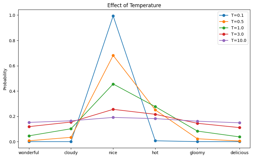
The effect of temperature to the resulting probability distribution
The model may produce the nonsensical output “Today’s weather is so delicious” if you set the temperature to 10!
Top-k Sampling
The model’s output is a vector of logits for each position in the output sequence. The inference algorithm converts the logits to actual words, or in LLM terms, tokens.
The simplest method for selecting the next token is greedy sampling, which always selects the token with the highest probability. While efficient, this often yields repetitive, predictable output. Another method is to sample the token from the softmax-probability distribution derived from the logits. However, because an LLM has a very large vocabulary, inference is slow, and there is a small chance of producing nonsensical tokens.
Top-$k$ sampling strikes a balance between determinism and creativity. Instead of sampling from the entire vocabulary, it restricts the candidate pool to the top $k$ most probable tokens and samples from that subset. Tokens outside this top-$k$ group are assigned zero probability and will never be chosen. It not only accelerates inference by reducing the effective vocabulary size, but also eliminates tokens that should not be selected.
By filtering out extremely unlikely tokens while still allowing randomness among the most plausible ones, top-$k$ sampling helps maintain coherence without sacrificing diversity. When $k=1$, top-$k$ reduces to greedy sampling.
Here is an example of how you can implement top-$k$ sampling:
|
1 2 3 4 5 6 7 8 9 10 11 12 13 14 15 16 17 18 19 20 21 22 23 24 25 26 27 28 29 30 |
import matplotlib.pyplot as plt import torch import torch.nn.functional as F
vocab = [“wonderful”, “cloudy”, “nice”, “hot”, “gloomy”, “delicious”] logits = torch.tensor([1.2, 2.0, 3.5, 3.0, 1.8, 1.0]) # (vocab_size,) scores = logits.unsqueeze(0) # (batch, vocab_size) k_candidates = [1, 2, 3, 6]
fig, ax = plt.subplots(figsize=(10, 6)) for top_k in k_candidates: # 1. get the top-k logits topk_values = torch.topk(scores, top_k)[0] # 2. threshold = smallest logit inside the top-k set threshold = topk_values[..., –1, None] # (…, 1) # 3. mask all logits below the threshold to -inf indices_to_remove = scores < threshold filtered_scores = scores.masked_fill(indices_to_remove, –float(“inf”)) # convert to probabilities, those with -inf logits will get zero probability probs = F.softmax(filtered_scores, dim=–1)[0] # sample from the filtered distribution sampled_idx = torch.multinomial(probs, num_samples=1).item() print(f“Top-k = {top_k}, sampled: {vocab[sampled_idx]}”) # Plot the probability distribution ax.plot(vocab, probs.numpy(), marker=‘o’, label=f“Top-k = {top_k}”)
ax.set_title(“Effect of Top-k Sampling”) ax.set_ylabel(“Probability”) ax.legend() plt.show() |
This code modifies the previous example by filling some tokens’ logits with $-\infty$ to make the probability of those tokens zero. Running this code may produce the following output:
|
Top-k = 1, sampled: nice Top-k = 2, sampled: nice Top-k = 3, sampled: hot Top-k = 6, sampled: delicious |
The following plot shows the probability distribution after top-$k$ filtering:
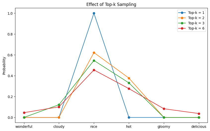
The probability distribution after top-$k$ filtering
You can see that for each $k$, the probabilities of exactly $V-k$ tokens are zero. Those tokens will never be chosen under the corresponding top-$k$ setting.
Top-p Sampling
The problem with top-$k$ sampling is that it always selects from a fixed number of tokens, regardless of how much probability mass they collectively account for. Sampling from even the top $k$ tokens can still allow the model to choose from the long tail of low-probability options, which often leads to incoherent output.
Top-$p$ sampling (also known as nucleus sampling) addresses this issue by sampling tokens according to their cumulative probability rather than a fixed count. It selects the smallest set of tokens whose cumulative probability exceeds a threshold $p$, effectively creating a dynamic $k$ for each position to filter out unreliable tail probabilities while retaining only the most plausible candidates. When the model is sharp and peaked, top-$p$ yields fewer candidate tokens; when the distribution is flat, it expands accordingly.
Setting $p$ close to 1.0 approaches full sampling from all tokens. Setting $p$ to a very small value makes the sampling more conservative. Here is how you can implement top-$p$ sampling:
|
1 2 3 4 5 6 7 8 9 10 11 12 13 14 15 16 17 18 19 20 21 22 23 24 25 26 27 28 29 30 31 32 33 34 35 36 |
import matplotlib.pyplot as plt import torch import torch.nn.functional as F
vocab = [“wonderful”, “cloudy”, “nice”, “hot”, “gloomy”, “delicious”] logits = torch.tensor([1.2, 2.0, 3.5, 3.0, 1.8, 1.0]) # (vocab_size,) scores = logits.unsqueeze(0) # (1, vocab_size)
p_candidates = [0.3, 0.6, 0.8, 0.95, 1.0] fig, ax = plt.subplots(figsize=(10, 6)) for top_p in p_candidates: # 1. sort logits in ascending order sorted_logits, sorted_indices = torch.sort(scores, descending=False) # 2. compute probabilities of the sorted logits sorted_probs = F.softmax(sorted_logits, dim=–1) # 3. cumulative probs from low-prob tokens to high-prob tokens cumulative_probs = sorted_probs.cumsum(dim=–1) # 4. remove tokens with cumulative top_p above the threshold (token with 0 are kept) sorted_indices_to_remove = cumulative_probs <= (1.0 – top_p) # 5. keep at least 1 token, which is the one with highest probability sorted_indices_to_remove[..., –1:] = 0 # 6. scatter sorted tensors to original indexing indices_to_remove = sorted_indices_to_remove.scatter(1, sorted_indices, sorted_indices_to_remove) # 7. mask logits of tokens to remove with -inf scores_processed = scores.masked_fill(indices_to_remove, –float(“inf”)) # probabilities after top-p filtering, those with -inf logits will get zero probability probs = F.softmax(scores_processed, dim=–1)[0] # (vocab_size,) # sample from nucleus distribution choice_idx = torch.multinomial(probs, num_samples=1).item() print(f“Top-p = {top_p}, sampled: {vocab[choice_idx]}”) ax.plot(vocab, probs.numpy(), marker=‘o’, label=f“Top-p = {top_p}”)
ax.set_title(“Effect of Top-p (Nucleus) Sampling”) ax.set_ylabel(“Probability”) ax.legend() plt.show() |
Running this code may produce the following output:
|
Top-p = 0.3, sampled: nice Top-p = 0.6, sampled: hot Top-p = 0.8, sampled: nice Top-p = 0.95, sampled: hot Top-p = 1.0, sampled: hot |
and the following plot shows the probability distribution after top-$p$ filtering:
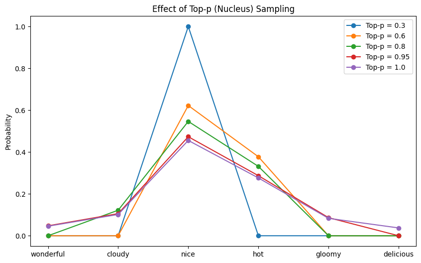
The probability distribution after top-$p$ filtering
From this plot, you are less likely to see the effect of $p$ on the number of tokens with zero probability. This is the intended behavior as it depends on the model’s confidence in the next token.
Further Readings
Below are some further readings that you may find useful:
Summary
This article demonstrated how different sampling strategies affect an LLM’s choice of next word during the decoding phase. You learned to select different values for the temperature, top-$k$, and top-$p$ sampling parameters for different LLM use cases.